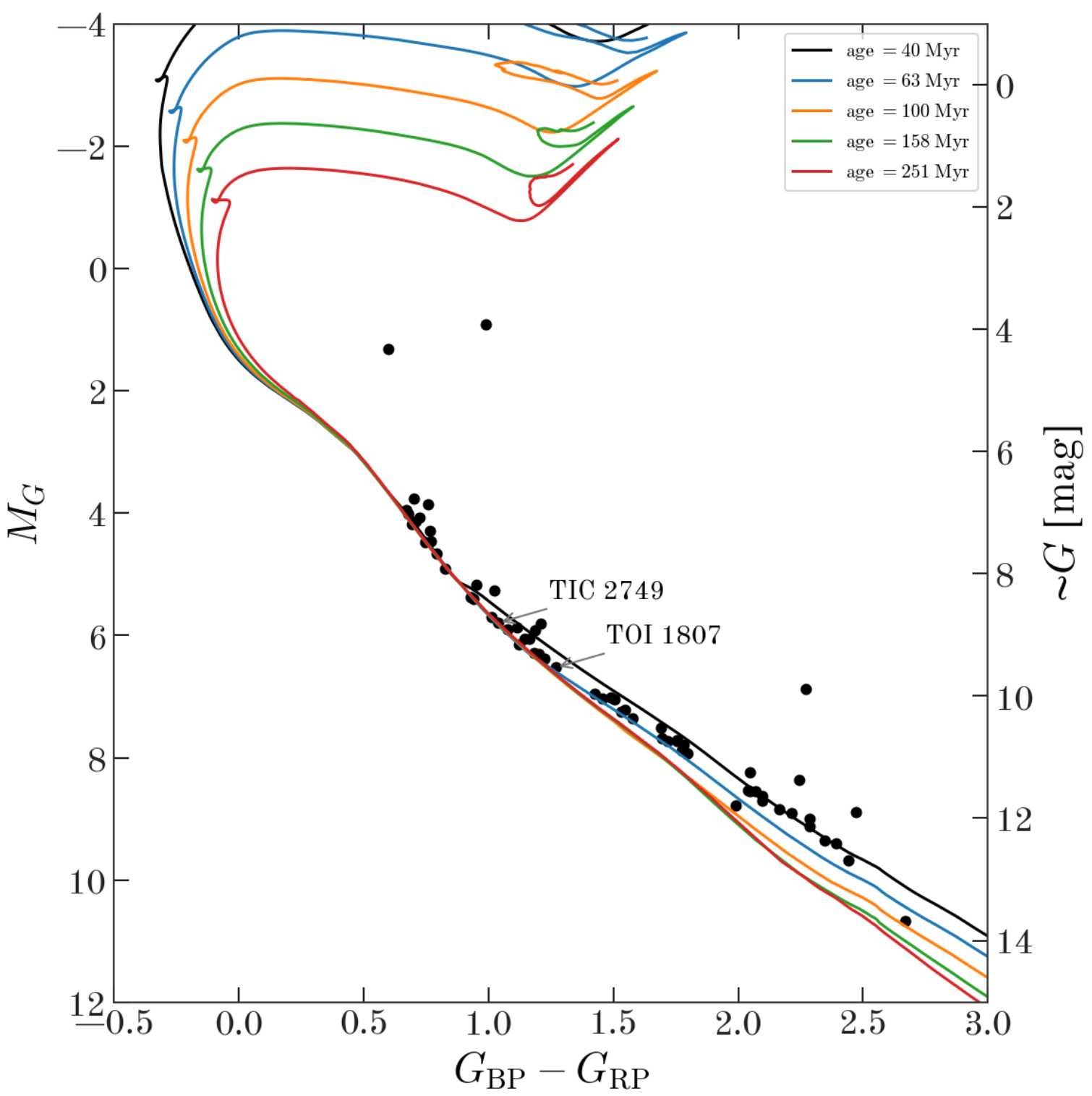
Adrian Price-Whelan and Christina Hedges started off this week’s meeting with an update about the new nearby moving group that they found when looking into the pair of transiting planet systems that they discussed three weeks ago. The header figure of this post shows a color-magnitude diagram showing the likely moving group members that they identified using Gaia radial velocities and proper motions. Christina and Adrian have compiled compelling evidence that these stars are members of a previously unknown, youngish (100 Myr), nearby (~40 pc) moving group. One feature that you might notice in the above figure is that the main sequence seems to be truncated at the bright end. Adrian and Christina hypothesize that this is caused by Gaia DR2’s bright limit for radial velocities. There was some discussion of the fact that this means that some bright (naked eye?) stars might be members of this group.

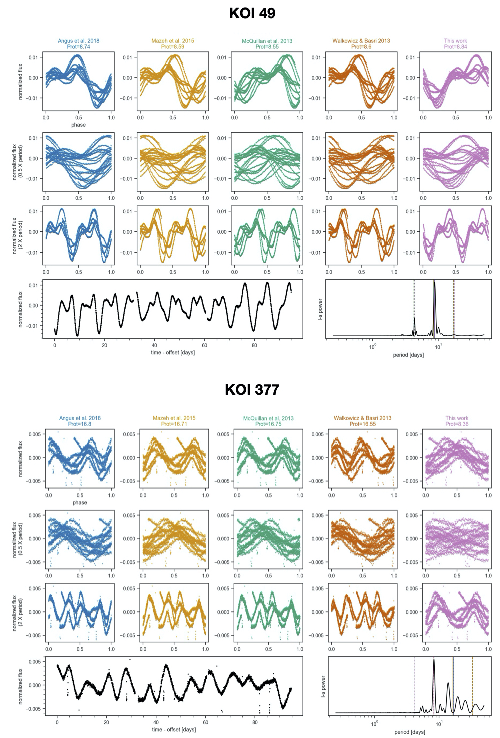
Next, David W. Hogg asked the group for feedback on a possible undergraduate project idea where the student would look at the TESS light curves for the binary systems discovered by Price-Whelan et al.. There was some discussion about what features would be expected in these light curves (eclipses, ellipsoidal variations, rotation signatures, etc.). The group had various ideas of interesting things to study, such as limb-darkening profiles as a function of effective temperature and spun up primary stars in close binaries.

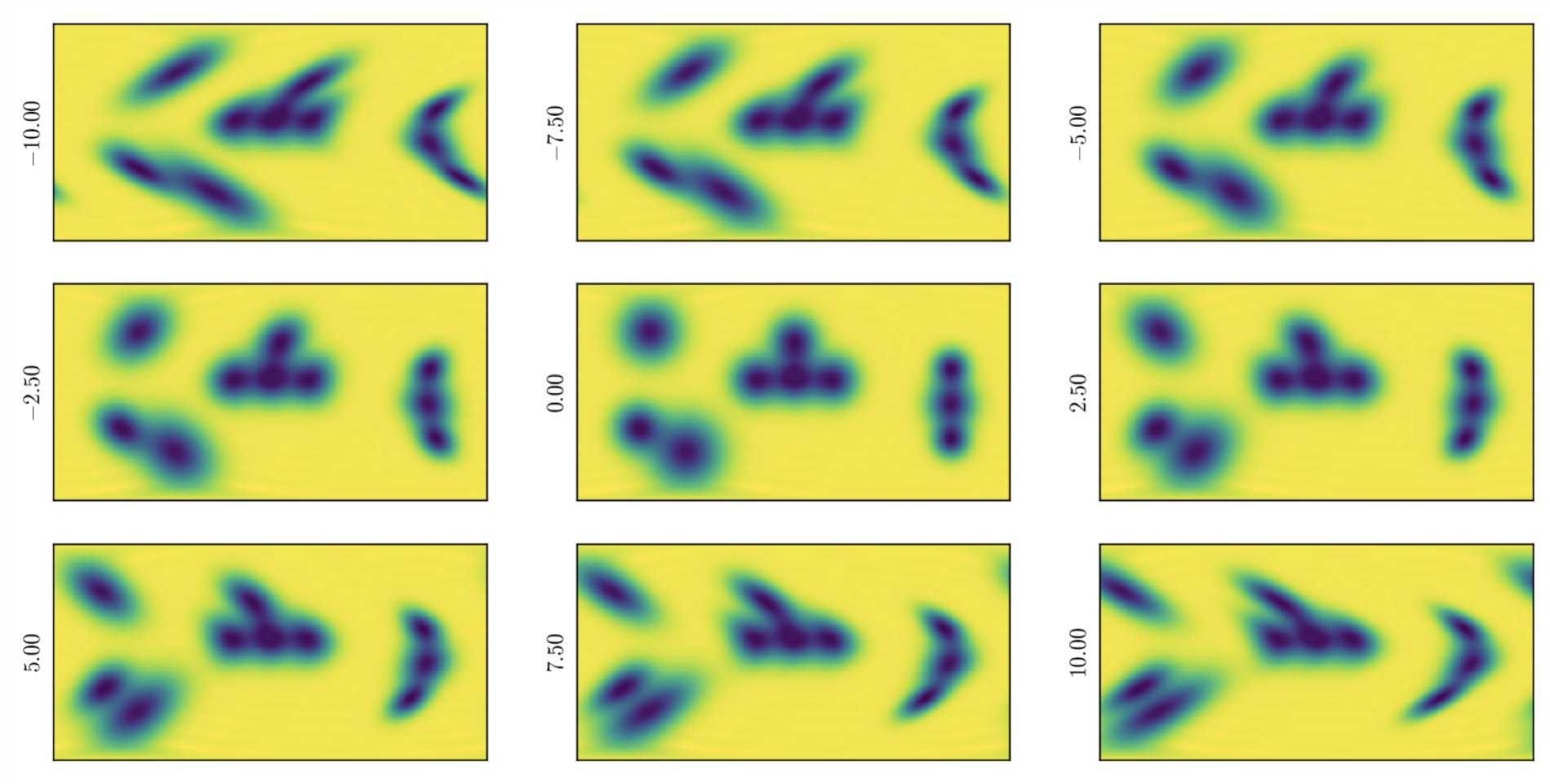
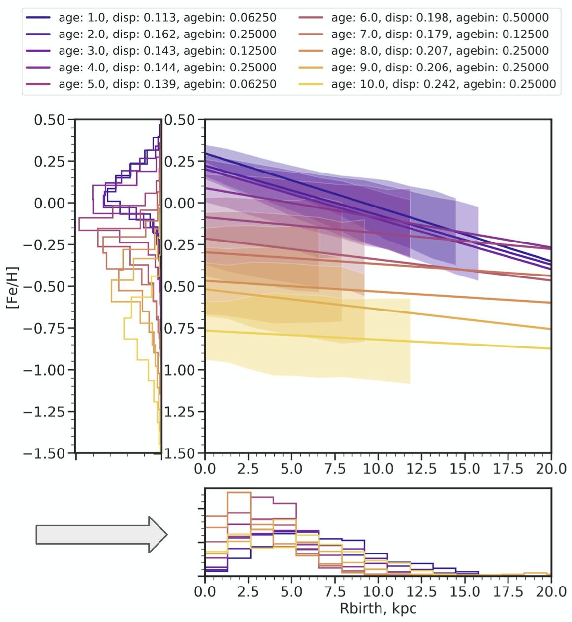
Then, Ruth Angus showed some interactive figures that she made using Bokeh based on results from Lucy Lu (Columbia & AMNH) who has been developing a method to estimate stellar ages using their Galactic kinematics. The technique currently depends on binning stars in color, magnitude, and rotation period space. Ruth and Lucy have been investigating how their results depend on the choices made in this binning procedure. The group suggested that perhaps this could be recast as a huge hierarchical model where the velocity distribution (instead of the velocity dispersion) is represented as a non-parametric function of these same parameters, but this would still require choices about representation that might not be easier.

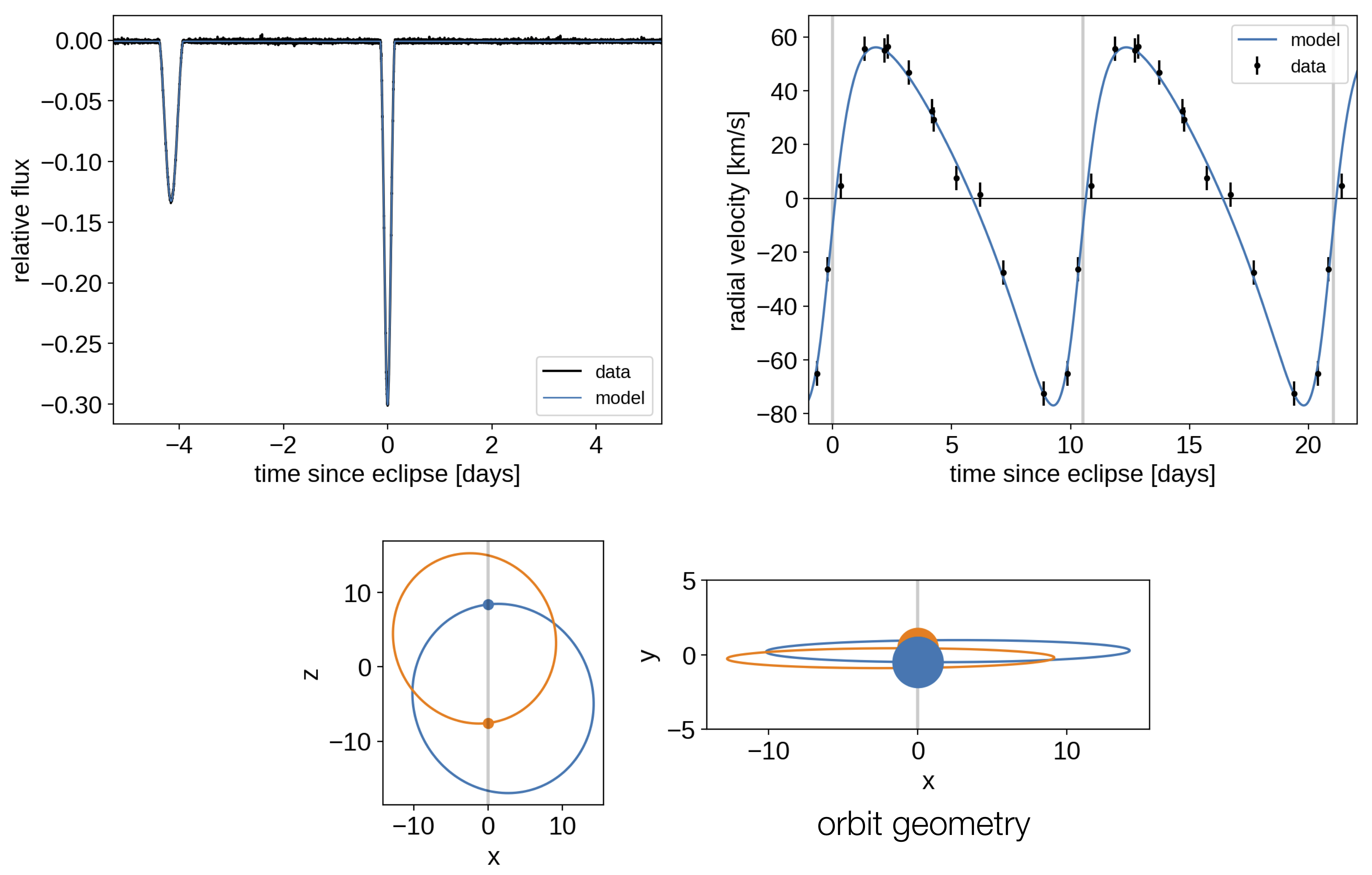
Finally, I shared a data analysis challenge that Trevor David brought to me. He is fitting astrometric observations of a binary star system with an orbital period that could be on the order of 100 years. Needless to say, the phase coverage of the observations is not great (although they do have a longer than 20 year baseline). Trevor has been using my exoplanet code and following the astrometry tutorial, but finding some painful degeneracies between parameters (especially tricky is the phase of periastron passage). There was a discussion of possible reparameterization choices, including using a series expansion of the orbit as a function of time to choose reasonable parameters. It was also suggested that we could try a rejection sampling method like the one developed by Sarah Blunt for the obitize code, but I think it will be possible to come up with a more efficient scheme in this particular case.

This week’s meeting started with an update from Rodrigo Luger about his work to map the surfaces of stars using phase curves and occulations. In particular, he has been working on techniques for increasing the efficiency of his methodology when the nullspace of the problem is large or, in other words, when very little information is actually available in the light curve. He has discovered a technique that is similar to previous work by Emily Rauscher where it is possible to re-cast the inference problem into the (much lower dimensional) subspace where the data are constraining, thus drastically reducing the computational cost. However, it seems like this improvement no longer applies if we want to actually generate the distribution over surface maps that are consistent with the data. It was suggested that it might be possible to generate these maps as a post-processing step, after fitting for all the other parameters of the system.

Next, Emily Cunningham updated the group on her project to disentangle the accretion history of the Milky Way stellar halo by modeling the abundance distribution of halo stars using templates built from observations of dwarf galaxies. She has preliminary results looking at a set of Milky Way-like simulations which provide an idealized test for the methodology. The header figure shows examples of some of the templates that she is using. However, since the model Emily is currently using just models the current abundance distribution as a linear combination of these templates, the interpretation of the results can be a little tricky. In particular, she is interested in determining the number and distribution (in, say, stellar mass and age) of the accretion events that assembled the halo. There was some discussion about the possibility of applying some sort of non-parametric mixture-of-templates model to make this measurement.

Then Kate Storey-Fisher shared some results from her project to detect anomalous galaxies in survey images using deep learning. Kate previously blogged about this project so you can check that post out for more details. Since that post, Kate has been developing an auto-encoder, trained on the residuals between the data and the GAN predictions for each galaxy, that she can then use to determine how “anomalous” each galaxy really is. In this context, the auto-encoder is acting as a dimensionality reduction that identifies features that seem to do a good job of ordering the the galaxy images in terms of how typical they are. There was some discussion about the possibility of skipping the GAN step in the process and directly applying the auto-encoder to the observations, but it’s possible that this wouldn’t perform as well since the GAN does a good job of building a distribution over the population of expected galaxy images.

Next, Trevor David shared three versions of a plot that he is making for a paper. He has taken high-resolution, time series spectroscopy of a transiting exoplanet (or, more specifically, its host star) and identified some excess variability in the red wing of the H-alpha line, in the out-of-transit data. This variance is close to a narrow telluric feature and the significance is low, but high enough to be interesting, so it is a bit tricky to demonstrate exactly what is being observed. The group had many opinions about the choices made in these plots and gave suggestions for improving the clarity.

Finally, we finished the meeting with a discussion, led by John Forbes, about the merits and costs of packaging and documenting code from a research project that is niche but potentially useful to other researchers. The argument was made that the most impactful scientific software will probably be simple (very good at exactly one thing) or extremely flexible (with all the possible knobs). Author’s note: I would argue, that perhaps there’s one other mode: a good “plugin” interface so that users can implement the knobs they need. But perhaps that falls into the second catagory anyways… In contrast, there was also a discussion of the fact that sometimes its not possible to predict all the potential use cases of your code and there are some examples where research code has been successful repurposed for related, unexpected applications. We did not come to any real conclusion about whether or not packaging and documenting all research code is worth it (I think it is!), but it was some good food for thought.

David W. Hogg started out this week’s group meeting by sharing a project that he has been working on with Anna-Christina Eilers (MIT) to understand the systematic effects in stellar abundance measurements made by the APOGEE survey. They start with the (not totally justifiable) assumption that, while abundance will be a function of birth location, it should not be a function of evolutionary state. While this is observed for some elements (iron, for example) there are clear trends of calcium abundance with surface gravity in the APOGEE sample. This could the result of systematics or the fact that the observed abundance patterns for evolved stars will not be the same as their birth abundances. David W. and Anna-Christina are interested in deriving a non-parametric method for determining birth abundances from the current observed abundances and an estimate of the Galactocentric positions.

Next, Christina Hedges (NASA Ames) and Adrian Price-Whelan shared an interesting TESS discovery: a pair of nearby, young transiting planetary systems whose hosts were previously shown to be in a widely-separated co-moving pair. One of these targets hosts three transiting planets and is already already interesting in its own right, but the fact that it is in a co-moving pair with another transiting planet host makes this a potentially very important benchmark system. Christina and Adrian also have some preliminary evidence that these two stars might be members of a larger (previously unidentified) association. We discussed the fact that, especially if their masses are accessible by radial velocity, these planets could be very useful for comparative studies of planet formation and evolution.

Rodrigo Luger shared some work that he has been doing (also in collaboration with Christina Hedges) to measure stellar differential rotation and star spot evolution timescales using precise photometric time series. Using an extension of his starry method, Rodrigo has developed a computationally tractable method for inferring the statistics of the time-variable surface map of a star based on its rotational phase curve in integrated light. This measurement is extremely degenerate, partly because of physics (spot evolution and differential rotation can produce very similar light curves) and partly because of math (there are some parts of the system, called the null space, that just can’t ever be measured). But, Rodrigo has some very impressive results that demonstrate that he can recover robust inferences for the differential rotation shear and spot evolution lifetimes using a non-parametric model.

Kate Storey-Fisher shared some figures from a paper that she is working on where she has developed a novel estimator for the correlation function of galaxies. Traditionally these measurements are made by binning the measurements on different angular scales, but Kate has developed a class of methods that don’t require binning. Instead the correlation function is described by a set of smooth basis functions and the estimation procedure involves measuring the weights of these functions based on the data. Kate has demonstrated (using simulations) that this method produces lower variance and less biased estimates of the correlation function than the standard method, even when the model is much less flexible. One of these figures is shown at the top of this post and there was some discussion about color choices (what do you think?) and how to best visually compare the different methods in a figure like this. In particular, the suggestion was made that perhaps this figure would be clearer as two panels rather than one.

Finally, I complained about coding in C++ and how hard I find some things that I would easily do in Python (like iterate over a tuple of arguments for an arbitrary function, don’t ask). The only useful thing that I shared was a link that I had discovered (only like 5 years late) when making my slide: carbon.now.sh a tool that makes cute screenshots of code like this.

In today’s meeting the group had a discussion about racism (in particular anti-Black racism) and our role as individuals and as a group in perpetuating it. This was an uncomfortable conversation for some group members and many of the more vocal members of the group (myself very much included) are not yet well-equipped to lead such a discussion. We spent some time sharing recommended reading lists, online educational resources, and brainstorming ideas for how to use this group to learn. In particular, we have committed to continuing these discussions in the future, recognizing that combating racism is an ongoing process. We discussed the possibility of a regularly-meeting reading group to learn about racism within astronomy and more broadly, but the specific structure of this group is still to be determined. There was some disagreement about the scope of this discussion and whether or not it is possible to focus on racism within academia.

As is often the case in such an environment, we were much more comfortable discussing institutional racism and brainstorming things we can do as a group to address this within our institution. While there was unsurprisingly nothing groundbreaking uncovered in this discussion, we identified several immediate action items (mostly in the context of hiring) and recognized that this is something that we also need to continue to learn about.

Finally, we shared links to the #strike4blacklives and #ShutDownSTEM initiatives that are organizing a virtual walkout next week where non-Black academics will take (at least) one day to educate themselves and take action towards eliminating racism. More information about these strikes, as well as recommended actions to take, can be found at the above links.

David W. Hogg started this week off by leading a discussion about how one might define a “discovery” in astronomy with a specific focus on the context of exoplanet detections in radial velocity surveys. This discussion was inspired by work he has been doing with Megan Bedell to make observing strategy recommendations for the Terra Hunting Experiment, an upcoming decade+ long survey to detect extrasolar Earth-analogs using extreme-precision radial velocities. One of the core questions is whether or not it is sufficient to define a detection as a precise, non-zero, measurement of the radial velocity amplitude. It might also be necessary to include a statement about the precision with which the other orbital parameters are measured. For example, a radial velocity “trend” might not qualify as a detection even if the lower limit on the amplitude is significantly non-zero. This led to discussions about whether or not marginalization is required for quantifying these detections at the limits of the survey detection threshold.

Next, Emily Cunningham shared a new project where she is using the Latte suite of Milky Way-like galaxy simulations to develop data-driven methods for understanding the assembly history of the Milky Way stellar halo. Following on earlier work by Duane Lee, Emily is working to construct a library of “template” distributions in the space of stellar abundances. These templates will be constructed by looking at accreted dwarf galaxies in the simulations and then Emily plans to model the mixed population using a linear combination of these templates to determine the relative contribution of different classes of accretion events to the assembly of the halo. After testing these methods on the simulations, Emily plans to determine which changes will be required to apply these methods to the observed stellar population even in the face of selection effects and realistic uncertainties. There was some discussion of how this methodology is similar to a low-rank matrix factorization problem and how this relationship could be used to develop a data-driven method for constructing the templates without sacrificing interpretability.

Then, Jiayin (DJ) Dong shared a project where she has measured the eccentricity distribution of warm giant planets detected using data from NASA’s TESS mission. After detecting and performing a detailed characterization of the transit light curves for a sample of about 80 warm giant planets, DJ is using “the photoeccentric effect” in a hierarchical Bayesian model to make robust inferences about the eccentricity distribution. This model is high-dimensional and the geometry of the problem can be pathological in some cases, making robust inferences tricky, but DJ has figured out these technical issues and has a working implementation in PyMC3. It is already clear that the eccentricity distribution of these exoplanets is multimodal (as seen in the header figure). The final inferences that DJ makes about this distribution will have a profound influence on our understanding of the evolution of planetary systems and she will be able to place constraints on the relative frequency of eccentric migration or in-situ formation channels.

Finally, I (Dan Foreman-Mackey) showed some plots that I have generated as part of a project in collaboration with Mariona Badenas Agusti (MIT) to revisit an interesting eclipsing binary system observed by Kepler and now TESS, using my exoplanet code. There are many technical aspects of this system that make it hard to model (there’s a lot of data and many parameters), but the physics is also non-trivial (the orbit is precessing, the stellar oscillations are coherent and measured at extremely high precision, etc.). I’m excited to get exoplanet working for this system, but I’m still struggling to get robust inferences in finite time.

This week we had a smaller group meeting than usual (long weekend, summer weather, apocalypse, etc.), but we still had some interesting conversations!

Rodrigo Luger discussed some work he’s been doing to efficiently fit the light curves of differentially rotating stars (see the header figure). This was inspired by his collaboration with Fran Bartolić to map the time variable surface of Io using occultation light curves as discussed last week. In the limit of long lived spots, Rodrigo has demonstrated that many of the degeneracies commonly found when mapping stellar surfaces using phase curves can be broken. But, he’s now looking for good test cases (including this sample) and he will look at the issues introduced by variable spot lifetimes.

Next, John Forbes updated the group on a project that he previously blogged about where he (in collaboration with Nia Imara, Harvard) is quantifying the density structure in turbulent box simulations. The key ingredient of their method is that the eigenvalues (or ratios thereof) of the local Hessian matrix of the density (or log density) seem to separate the structures in these simulations along axes corresponding to the qualitative descriptors that are generally used. Now they’re working to get a better understanding of how to interpret these quantities by visualizing the Hessian matrix at various points in this parameter space. These are hard to visualize since the data live in three dimensions so they have been making 3D matplotlib animations of the stencil used to estimate the Hessian, but they remain hard to interpret. There was some discussion about alternative visualization techniques and whether or not it even makes sense to try to qualitatively interpret these features.

David W. Hogg shared some work he has been doing with Soledad Villar (NYU) to understand the relative performance of discriminative and generative models for prediction tasks in several toy scenarios. They find that generative models marginally outperform discriminative models in many of the test cases they try. In particular, they find—in agreement of previous results in the literature—that discriminative models have catastrophically poor performance when the number of training samples is approximately equal to the dimension of the data, even when the model performs well for both fewer and more training points.

Finally, Sam Grunblatt led a discussion about the definition of the Galactic stellar halo. He asked about the relative importance of kinematics, chemistry, and current coordinates. There was broad agreement that chemical and dynamical arguments are both important, but the discussion predictably devolved into the assertion that the Milky Way is not multi-modal in any dimensions and that classifications should be continuous rather than discrete.

Given the current state of the world, we have been holding the Astro Data Group meeting virtually for the past couple of months and this blog has taken a hit over that time. This week, I (Dan) have decided to try to start posting a short summary of what we talk about each week so we’ll see how long I keep it up :)!

Fran Bartolić started us off with a discussion of how he is using non-negative matrix factorization to map the time variable surface of Io using occultation light curves. In particular, he’s modeling the time variable surface as a linear combination of starry maps where the coefficients vary as a function of time. The results of this inference are prior dependent so he presented some of the prior information that he is considering: non-negativity constraints, sparsity priors, and Gaussian processes to capture smooth time variability and volcano duty cycles. There was some discussion about including spatial priors that would favor contiguous features in each map (for example, individual volcanos).

Trevor David has been investigating long run times and divergences in his PyMC3 inferences. To handle difficult posterior inferences, he has been increasing the target acceptance statistic in the tuning phase of his PyMC3 runs, but still ends up with some small percentage of diverging samples and long run times. Some of these issues can be handled by re-parameterization, but Trevor has been looking at various diagnostics to try and understand the behavior of his sampler. One such diagnostic is the comparison of the empirical marginal energy distribution and the conditional energy distribution (see figure 23 of Betancourt 2017 for an example), and Trevor finds a small skew in these distributions (with heavier tails to larger energies).

On a related topic, I presented some work I have been doing to improve the tuning performance for PyMC3 when there is a large dynamic range in posterior precision across dimensions. The idea is fairly simple—set the target acceptance statistic to something low (like 50%) at the beginning of the tuning phase and increase this target to the final value throughout tuning—but it seems to work well for at least some test cases. This is currently implemented in exoplanet, but more testing will be needed before this is ready for prime time.

Dreia Carrillo shared the figure at the top of this post and asked for feedback about its clarity and, in particular, the binning choices made in the bottom histogram. This figure shows stellar metallicity gradients as a function of birth radius in a Milky Way-like galaxy simulation. The main panel shows how these gradients change as a function of age, but doesn’t capture underlying density of stars so she included the histograms to show this distribution, and specifically to highlight the signatures of inside-out disk formation. The group discussed options for making the birth radius histogram plot clearer. These suggestions included using a kernel density estimate instead of a histogram and using fewer, wider age bins.

To finish, Emily Cunningham led a discussion of how members of the group manage their time when working on multiple parallel projects and how to identify when we are over-committed to too many projects. The group agreed that this is something we all struggle with, especially since we are currently all working in isolation. Group members have devised some tactics for dealing with this, including setting goals on week-long time scales instead of daily or by running work by collaborators more frequently. We also discussed the fact that side projects and context switching can be useful (especially these days) to help getting ourselves out of a research rut or to identify our next projects, even if they don’t always lead to visible results.

A common problem with algorithmic determination of rotation periods from light curves is that the “best” period may actually be the undertone/subharmonic or harmonic of the true period (in other words, twice or half the true period). Two real examples from the Kepler mission are shown here.

In the first row of each figure, the Kepler light curve of a star is phase-folded on a period either from the literature or determined using a Lomb-Scargle (L-S) periodogram. In the second and third rows, the light curve has been phase-folded on half and twice the period in the first row, respectively. The bottom two panels show the light curve from a single Kepler quarter and the periodogram itself.

With KOI 49, the various estimates for the rotation period are in agreement, and it seems clear that those estimates are correct. Why? We see two peaks (and troughs) in the phased light curve of uneven height. The simplest explanation for this behavior is a fairly stable arrangement of two dominant spot groupings of different size and/or contrast on the surface. Reality is definitely more complicated, but the light curves of many stars can be approximated with a two-spot model.

For KOI 377, the literature period estimates (first four columns) are in agreement, while the L-S method (last column) prefers approximately half of that period. It’s worth noting here that the L-S method assumes a sinusoidal model for the data and has indeed selected the period which best approximates the data as a sinusoid. What’s going on?

Imagine this pathological case: a star with two spots equal in size, contrast, and latitude but separated by 180 degrees in longitude, spinning on an axis perpendicular to our line-of-sight. As this star rotates, an observer would record a light curve showing two peaks and two troughs of exactly equal height/duration, and would not be blamed for reporting the rotation period as half the true period.

What is the correct period for KOI 377? From the plot it’s not immediately clear. However, other clues exist in the light curve. Compared with KOI 49, the light curve is less “stable” and shows variations about twice as small in amplitude. From ensemble studies of Kepler light curves it’s known that rotation period is anti-correlated with variability amplitude, and differential rotation (which traces “stability”) correlates with stellar mass, which itself correlates with rotation period. So, one path towards determining more reliable rotation periods may rely on all available information, such as the variability amplitude and stellar parameters. In fact, group members Lucy Lu and Ruth Angus are working on just this problem with Astraea.

At the TESS Ninja 3 workshop, Jessica Birky (UW) cross matched Adrian’s catalog of binary star systems found using APOGEE with the TESS 2-minute cadence light curves and found a handful of light curves with eclipses. With APOGEE cadence, it can be hard to tie down the period of the orbit, but a TESS light curve can approximately perfectly measure the period, epoch, and inclination of the orbit. This breaks degeneracies in the orbital solution and can lead to precise contraints on the stellar parameters. At the workshop, I worked with Birky and others to start fitting these orbits and since then I added support for eclipsing binary light curves directly into exoplanet (the code). The figure this week shows an initial fit for one of these targets. This one is interesting because the deeper eclipse seems to actually be the secondary; the star being eclipsed during the shallower event is actually brighter, but the orbital configuration (specifically the inclination and eccentricity) is such that this produces a shallower signal. This falls out of light curve only fit (the flux ratio is required to be >1) and is consistent with the radial velocity measurements (APOGEE only measures one set of velocities—presumably for the brighter star). The top panels show the TESS light curve and APOGEE radial velocities and the bottom panels show the best fit orbital configuration (the observer is at z = infinity) with the configuration during the deepest event shown with the radii drawn to scale. I haven’t been able to get the MCMC to run efficiently for this yet (probably because of parameterization issues), but hopefully we’ll have a fully working system soon!

Inspired by a conversation with Andy Casey who we visited at Monash University in Melbourne last week, I decided to write a Collaboration Policy, and share my feelings on the topic at our weekly group meeting.

At Monash, Andy showed me the Research Expectations page of his website, which is a document outlining the expectations he has for his students, and what their expectations might be for him. I love this idea and would like to create my own research expectations guidelines for any students working with me, current or future. As I started to write it however, I realized I wanted to write a zeroth-order expectations document first. Something a little more general, targeted at everyone I work with: a collaboration policy.

My collaboration policy document states what expectations I have for co-authors on my papers, and what they should expect from me as a co-author on their papers. It describes how I select and order co-authors, how I like the commenting and feedback procedure to go, etc.

The document also outlines an explicit policy for proposal, as well as paper, collaboration, including my definition of the responsibilities of funded and unfunded collaborators. This is something that I have found particularly difficult to navigate in the past, because proposal authorship and responsibility distribution can be delicate and political. I found it really helpful to make my expectations explicit and I’m sure it will help avoid a few awkward conversations in future.

Finally I outline my philosophy on authorship. For example, I feel strongly that “whomever does the work leads the paper”, a policy that may seem obvious but still, sadly, has to be made explicit on occasion.

This is just a first version, and there’s a lot more I’d like to add. The Astro Data group were enthusiastic about working on a collaboration policy together, and I think we’ll converge on an official version soon.

I really enjoyed writing this document. I’ll find it useful to send to my collaborators, but I also enjoyed solidifying some of my feelings and opinions on this topic. I recommend that everyone goes through this exercise!