At this week’s meeting I shared an update about a project called PyTorchDIA led by James Hitchcock (St. Andrews) where we are looking into how numerical tools developed for machine learning can be applied to astronomy. Unlike many applications of PyTorch, TensorFlow, etc. in astronomy, I’m not talking about using neural networks. Instead, I’m talking about using PyTorch to compute fast convolutions and matrix-vector products to accelerate more “traditional” astronomy problems. This is somewhat similar in spirit to the wobble project led by Megan Bedell (that strangely has never appeared on this blog, Megan!).

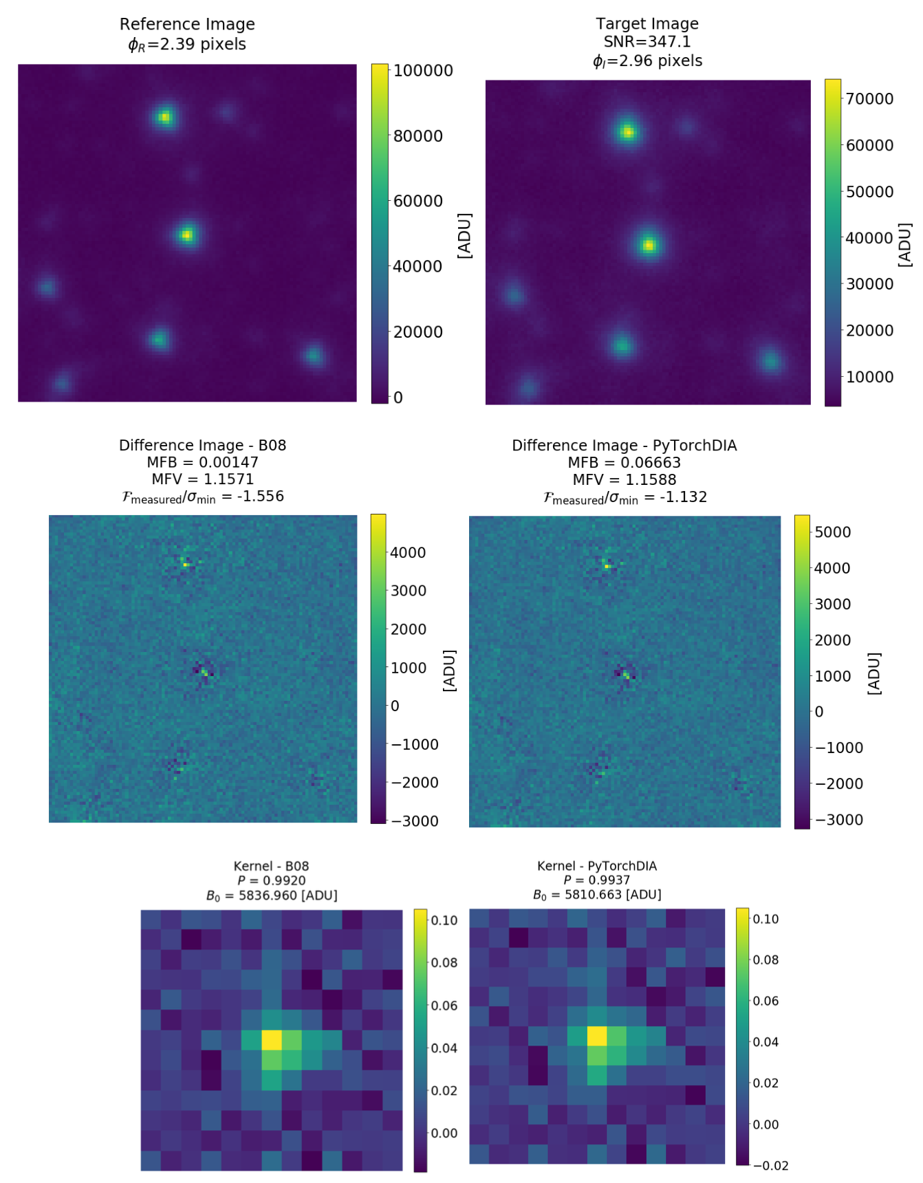
For the PyTorchDIA project, James and I realized that we might be able to easily port existing difference imaging methods to run on the GPU using PyTorch since the bottleneck operation is solving a large linear problem where the design matrix is a convolution. This is exactly the type of operation encountered in deep learning applications and exactly what frameworks like PyTorch are designed for. James took this one step further, and instead of directly solving this linear system, he uses an iterative solver that only requires matrix-vector products (rather than a full Cholesky factorization). This allows us to relax some of the assumptions (like Gaussianity of the observation model) of the standard methods so that we can use a robust loss function instead of sigma clipping.

Using the GPUs available on Google Colab, James finds that his method is at least an order of magnitude faster than optimized implementations of other commonly used methods for difference imaging, across a wide range of realistic test cases. We will hopefully be submitting this paper in the next week or so and we are already planning on incorporating this method into the pipelines for several existing and upcoming difference imaging surveys. But, the real reason why I shared this with the group was that I believe that there are some (potentially) useful lessons learned:

1. Astronomical imaging analysis shares a lot of structure with machine learning problems; let’s take advantage of that!
2. Some of the linear problems that we work on in the group might be easier and faster to solve if we use iterative solvers rather than direct solvers. The scaling is different, but also the implementations have been optimized for the forward calculation and these methods can open the possibility of generalizing the loss function.

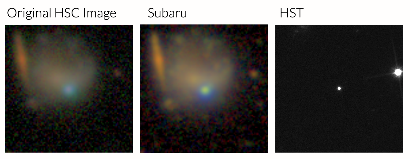
Aside: I also want to mention the awesome website weirdgalaxi.es (yes that is the domain name, but don’t click on that if you’re using Safari) that Kate Storey-Fisher made (and shared at this week’s meeting) as a continuation of the project that she previously blogged about.

After arriving at CCA a few weeks ago, I’m starting on a project with Adrian Price-Whelan and David W. Hogg. We are trying to figure out how to answer the question: What does it mean that APOGEE doesn’t have a bunch of binary systems containing black holes? Barring the obvious reason that APOGEE’s targets are low-ish mass stars and thus unlikely to be companions to BHs and their high-mass progenitors, we think it will be interesting to compare a bunch of synthetic binary populations generated with COSMIC to Adrian’s close binary catalog.

Step 0 of this process is to work out how to generate mock APOGEE catalogs with COSMIC data. This means I need to do real astronomy to convert the effective temperatures and bolometric luminosities in my simulations to (gasp) magnitudes of both the absolute and apparent kind. Luckily for me we found Tim Morton’s isochrones package that provides interpolated bolometric corrections from the MIST bolometric correction tables. The figure above shows a CMD that I made from a little test sample of a few synthetic binaries that follow the age and metallicity distribution of the m12i galaxy in the Latte Suite of the FIRE cosmological simulations. I was pretty excited to see the suuper obvious double main sequence and that COSMIC produced something that looks somewhat similar to what you’d expect (see e.g. Fig 5 here).

Steps 1 onward will include picking which kinds of binary interactions will most severely impact a BH + star population that APOGEE can see (hello BH natal kicks!) to set up our binary evolution model set and including dust extinction. I’m sure eventually I will also open real astro data files that at some point intheir distant post-processing past came from telescopes!

I’ve been working (slowly but surely) on an open source code extrabol which estimates the bolometric light curves of supernovae from an arbitrary set of filtered photometric observations. This code is based on a package by Matt Nicholl, SuperBoL.

Estimating the bolometric luminosity and black body temperature of a supernova is an extremely common analysis problem in time-domain astronomy as it allows astronomers to easily probe supernova explosion dynamics. Unfortunately, supernova light curves are often poorly sampled across multiple photometric filters, making it challenging to build a pseudo-bolometric light curve directly from the data.

In order to solve this problem, extrabol uses a 2D Gaussian process to extrapolate the supernova spectral energy distribution (SED) as a function of both wavelength and time. Extrabol is linked to the Spanish Virtual Observatory, a database of nearly every commonly used astronomical filter. Given the name of a telescope/filter, extrabol will link the observation to an effective wavelength. Using an arbitrary set of filters from the user, extrabol will estimate the underlying SED and then use this SED to estimate a black body temperature and radius. Eventually, the goal is to have extrabol linked with the Open Supernova Catalog, so that a user type in the name of a supernova and quickly build a bolometric light curve using public data.

For now, I am still working out some bugs! The Figure above shows an example light curve for a core-collapse supernova. Each observation is shown as a point (with error bars being smaller than the points). The GP interpolation is shown as lines, with uncertainty shown as shaded regions. Currently, I am assuming a mean function of a very dim magnitude, which works well before and after the supernova itself; however, if there is a large gap of data, the GP prefers artificially low luminosities. I got some very useful feedback from the Astro Data Group this week to investigate a more physically meaningful mean function, with residuals being modeled by the GP. My next step is figuring out if there is such a function which can be used for all flavors of supernovae!

At AstroHackWeek 2020 last week, a fight broke out - not between the supportive and friendly participants, but between emulators. I pitched a hack project on comparing emulation methods, mostly so I could show this emu vs. kangaroo fight video during my pitch, and a team of fighters assembled. All credit for this project shared with Catarina Alves, Johannes Heyl, Yssa Camacho-Neves, and Johnny Esteves!

One of my research projects is on emulating galaxy clustering statistics for speedier, more accurate inference of cosmological and assembly bias parameters. I had been wanting to try out different emulation methods on this data, as well as write up a pedagogical tutorial on emulation. In brief, emulators are regressors that imitate more complex models or simulations. They are trained on a limited set of simulation inputs and output and learn the layout of this (often high-dimensional) parameter space; then for any new set of inputs, they can quickly spit out output values, without performing a physical calculation or a full simulation.

Our hack team first wrote up a detailed explanation of emulators, complete with an example about a computational emu biologist; check it out in our complete tutorial here. Then we wanted to actually build some emulators and test them on astronomical data. My full-scale research dataset proved unwieldy for a week-long project, so I generated a set of two-point correlation functions using nbodykit. The winning emulator should be able to take the input values of (Omega_m, sigma_8, Omega_b) and predict the correlation function in each of 10 separation bins.

Each team member took on a different emulation framework. So far, our lineup includes an Artifical Neural Network, a Random Forest, a Decision Tree, and a Support Vector Machine (with Gaussian Processes on the way). The fighters tuned their implementations and hyperparameters to the best of their abilities. The fight was heated, with the emulators racing to train and test out their clustering predictions. You can see the predictions of the SVM compared to the true correlation function in the figure above.

To see the outcome, you’ll have to follow the full battle at The Great Emu Fight notebook. But the takeaways were:

• The Support Vector Machine emerged as the clear winner in accuracy for every metric we tested, emulating the correlation function to within a tenth of a percent for most r-bins. The Artificial Neural network came in a close second. (The second figure above shows the R^2 error; you can see the large difference in accuracy between the SVM and ANN compared to the DTree and RF.)
• However, the SVM was by far the slowest to train. The Decision Tree handily won the training round.
• The Decision Tree and the ANN were the winners when it came to prediction time (this is super important for inference!).
• The Random Forest was an all-around loser, being very slow at prediction and sadly inaccurate; we love and appreciate it anyway.
• Most importantly, all of these results are super dependent on emulator implementation, hyperparameter tuning, data normalization, and the dataset itself! So the reigning champion likely won’t reign for long.
• We built this project to be incredibly modular, so you can throw your own emulator or dataset into the ring. Follow one of our standalone notebook tutorials and tune the hyperparameters to improve on our results, or add in your own complete implementation, and join in the fight.

Check out the project in this repo, and follow the complete fight at The Great Emu Fight notebook. Huge thank you to the emu-fight team and the AstroHackWeek organizers!

Last week we had our first meeting of the new semester and we decided to try something “new”. In fact we went back to how we ran things back in the olden days: we take the total meeting time and divide it equally between people who are online, and everyone gives an update. In many ways, this is really how we want group meeting to go. The whole point is that, since group members work on such a broad range of topics, we want to have an opportunity to hear what everyone else has been up to. The goal is to identify shared interests and encourage collaborations across research areas.

This time (unlike the olden days), we had 18 group members (or collaborators working actively on a project with a group member) online (and that isn’t even the whole group these days - I’m not complaining!). This meant that even with 90 minutes, the updates had to be very short and the whole thing felt like quite a whirlwind (and I needed to take a nap after logging off). As a result, I’m not going to write up a summary of all the awesome work that folks are doing. Instead, I want to ask if anyone has advice or thoughts about running big group meetings like this.

Overall, it seems like the group appreciated this format, but agrees that it might be a bit overwhelming to do it every week. So the current plan is to proceed with the format from the summer (a shared slide deck where group members can choose to add a slide and then share a 10 minute update with some discussion) for most meetings, and then about once a month we would have a whirlwind update from everyone. I don’t love this option, because this meeting is often the only time that I get updates from many group members. But, we haven’t been able to identify a format that helps to make sure that everyone gets and opportunity to share. We’d love to hear if there are other groups out there doing interesting things with their meetings. We’re always keen to try experiments, especially since we’ll be staying fully-remote for the foreseeable future!

If you have thoughts, please Tweet at me or send me an email (should be easy to find!)

Jiayin Dong (DJ) updated us on her project to study the eccentricity distribution of warm-Neptune exoplanets discovered using data from the TESS mission. She has discovered and carefully characterized about 100 of these transiting planets. She then uses the “photoeccetric effect” to infer the distribution of eccentricities based on the observed distribution of effective “circular stellar densities”. The inferred distribution is the observed population of orbital eccentricities but, if the detectability of the planet is correlated with eccentricity, this won’t necessarily be equivalent to measuring the true intrinsic eccentricity distribution. This will be an important effect (eccentricity will scale with orbital period and the probability that a planet transits is also a function of its eccentricity), so DJ asked the group for recommendations about how to take this into account. This led to a discussion about “inverse detection efficiency” methods versus likelihood-based methods for population inference. (I have opinions about this… I’m writing this post so I’m allowed to editorialize!)

Next, John Forbes shared a data analysis challenge where he has a simulation of a forming galaxy where he has snapshots of several quantities that, to order of magnitude, should sum to satisfy a differential equation. In practice, because of numerics and approximations this differential equation is not exactly satisfied, so he is interested in fitting for, possibly time and space invariant, offsets or scales for each of these quantities to best fit the constraints. Currently, he is using linear least squares to fit for multiplicative factors (that don’t depend on time or position) for each quantity, but finds that the results are not satisfactory. Several suggestions were made for relaxing these assumptions and fitting a more flexible model. One option would be to fit multiple galaxies together (in some sort of hierarchical model) to propagate information between them. Another would be to allow use a Gaussian Process either to model residuals away from the least squares model or as priors on the coefficients that enforce smoothness in time and space.

Then, Daivd W. Hogg shared a first draft of a Mission Statement and 5-Year Plan for the Astronomical Data Group. These highlight some of the things that we think we do well (encourage better data analysis practices, develop and support open source software, etc.), but also identify some of the places where we want to spend more energy. The goal is to use these documents to help focus research areas and other group efforts, as well as hiring decisions.

Finally, I gave an update on the online.tess.science event (hackathon/sprint/something) that I am co-organizing. It starts on Sept 8 (just over one week from now!) and there will be nearly 150 participants from around the world. The header figure for this post shows the times that each participant is planning on being online during the 48 hours of the event - this really is a global experiment! We are working to find the right balance of unstructured, asynchronous time and synchronous social/networking/check-in time with the goal of encouraging participants to meet a broad range of other community members. Much of this, as well as our recommendations for how to navigate an event like this, is being codified in a “Participant Handbook” that I’ve drafted with my co-organizers. I expect that this document will continue to be useful for future events, even if they are in-person.

I started this week’s meeting by asking for feedback about our plans for the online.tess.science event that I am co-organizing in September. This event is the 2020 version (hopefully this is just a year, and not an indication that it will go up in flames) of the tess.science series of workshops where astronomers get together to collaborate on new projects related to NASA’s TESS mission. The previous 3 events have all been organized in-person and, since this event will be fully remote and international, there are various challenges (and opportunities) that we haven’t experienced before. One difference between this event and many other online conferences is that there will be no formal presentations. Instead, participants are encouraged to start new collaborations and try to learn something new. The group had a lot of good questions and feedback about our current plans. In particular, there was a good discussion about how important it will be to manage expectations, especially when people have experience with in-person events where they can walk across the room and ask questions of any other participant in real time. There were also some suggestions about how to encourage interactions between participants even if they are not directly collaborating. We’ll see how well we can execute on these plans!

Next, John Forbes discussed a data management/coding challenge that he’s currently facing. He has a large simulation where the properties of a set of about a million “particles” are saved to disk at a series of “times”. The output of this simulation can be thought of as a large multidimensional array where the first dimension is time, the second dimension is particle number, and the third indexes the various properties that are being tracked. This full dataset is too large to be loaded into memory and John wants to run an analysis on a subset of the most interesting particles at all times. However, since the data are stored as snapshots, loading the properties of a particular particle at all times is a computationally expensive task. Besides a few snarky comments about serialization formats, the group had several suggestions for how to improve this performance of this operation. The main observation was that the data are essentially stored in row-major order, while the operations would be more efficient on column-major ordered data. The group suggested several tools that could help here, including dask, Parquet, and Arrow.

And that was it… it is August, after all!

We had a quiet but interesting group meeting this week!

First, Trevor David shared some recent work with Gaby Contardo on looking at the exoplanet radius gap as a function of host star age and asked for feedback on methods for quantifying the gap width. He presented a few possible approaches, including fitting Gaussians to the 1D histogram of radii; fitting a line in the 2D radius-age plane by inverting the likelihood; or using a support vector machine model. We spent some time discussing what assumptions are being made in each of these cases. In particular, there was some debate about the validity of assuming Gaussian shapes for each of the two radius peaks. We also discussed the related problem of assigning individual planets to different sides of the radius gap. It might be necessary to perform the classification of data points in tandem with the characterization of the resulting gap in the distribution.

Next, Kate Storey-Fisher showed us an unusual galaxy in the Hyper-Suprime Cam data (pictured above). The HSC image of this galaxy was flagged by Kate’s GAN-based anomaly detection code, and archival data from Subaru and HST support its weirdness. Kate recently obtained a follow-up spectrum from Keck and she showed that the resulting placement of the source on the BPT diagram classifies it as a star-forming galaxy rather than an AGN. However, there are still some oddities, including possible markers of strong outflows. We spent time squinting through our Astronomer Goggles (TM) at the images and making extensive use of Zoom’s markup features. It’s always fun to dig into the data during data group meeting!

Finally, David W. Hogg showed us one of his quarantine projects: learning how to execute a perfect shuffle. He demonstrated that eight perfect shuffles in a row returns your deck of cards to the original ordering. This means that the permutation matrix corresponding to a perfect shuffle has the property that raising it to the eighth power returns the identity matrix. Linear algebra: it’s everywhere! We had a wide-ranging discussion covering combinatorics, psychology, and the entropy state of the universe. Our only real conclusion was that when playing poker with Hogg, you should insist on cutting the deck between shuffles.

We started this week’s meeting by discussing the possibility of organizing shared group meetings with other groups within CCA or within the broader astronomical community. While this group is focused on methodology, the scientific interests are broad so it could be useful to occasionally join forces with groups focused on specific research areas of interest to group members. It could also be useful as a method for encouraging random encounters between researchers who don’t normally overlap, especially while working remotely. Not everyone was completely enthusiastic about the idea, however, since there are already opportunities for group members to attend multiple group meetings within CCA and it might not be ideal to lose our one weekly meeting with the full group. It looks like we will try a test run with another group at CCA and, after that, consider options for future experiments like this.

Next, Ruth Angus asked for feedback on the project that she is proposing to the NSF Career program. She will be focusing on inferring rotation periods for stars using time series using data from the Zwicky Transient Factory and the Vera Rubin Observatory. There are many technical details from a time domain analysis side that she has been working hard on, but she was asking for feedback on the potential use cases for a huge catalog of rotation periods and gyrochronological ages for faint Milky Way stars. The group had many suggestions for applications and there was a good discussion of the project.

Rodrigo Luger talked about (gasp!) spherical harmonic representations of stellar surfaces and the resulting light curves. Building on the work he discussed last week, Rodrigo has worked out a better parameterization for the spherical harmonic expansion of spots on the stellar surface. He finds that if he parametrizes the spot using a Legendre polynomial expansion, all the spherical harmonic math that he needs to compute light curves turns out to be simple and the expansion of the spot is better behaved (no ringing and not going negative) than before. Furthermore, he has demonstrated that the time series Gaussian Process that he presented last week is the Gaussian density with the minimum K-L divergence to the distribution over stars with discrete spots. This has some interesting connections to variational inference.

Then, John Forbes shared a project where he is studying metal enrichment in Upper Scorpius. The data analysis problem that he presented is that he needs to infer the distances between a handful of stars and a specific molecular cloud, the potential site of enrichment. The projected distance (in the plane of the sky) is well measured, but John really needs the physical 3-dimensional distance and these stars only have noisy distance (from us) measurements. Therefore, he needs to marginalize over the line-of-sight distance when estimating his quantity of interest and he’s finding that the results are somewhat sensitive to his choice of prior for the 3-dimensional distribution of stars. There was some discussion about ideas for understanding this effect and making the best choices, but this conversation will have to also continue offline.

Adrian Price-Whelan and Christina Hedges updated the group on the project that they shared two weeks ago, where they had discovered a new young, nearby moving group. Since that meeting they have expanded their sample to include fainter and brighter stars that don’t have radial velocity measurements in the Gaia catalog. To determine membership probabilities, Adrian and Christina have implemented a probabilistic model that marginalizes over radial velocity when it is not measured. The resulting catalog has some contamination that can be removed using the RUWE metric from the Gaia pipeline. There are several bright (apparent magnitude of ~3) stars included in the cleaned sample and many fainter stars. The age estimates from isochrones, lithium abundance, and high-resolution spectroscopy all consistently suggest an age of about 200 Myr, but the new sample includes a non-trivial number of white dwarfs, which is a bit puzzling at that age. The suggestion was made that rotation periods might provide another good age estimate.

Finally, Sam Grunblatt asked for suggestions because he is running out of hard drive space for a project where he is currently generating millions of data files (including figures). There was some discussion of the relative merits of binary vs. ASCII formats for data products (use binary!), but Sam’s main issue is the huge number of plots that he’s saving. He generates these figures to make it faster and easier to page through and vet the results of a planet search using TESS. But, going forward he would like to automate this further so the recommendation was made that he avoid saving these figures for every target, restricting instead to the most “interesting” ones.

This week’s group meeting was a bit quieter than usual, but we still had some useful discussions.

Rodrigo Luger started us off with a discussion of a Gaussian Process kernel for light curves he has derived, using starry, that is parameterized by interpretable physical parameters of the target star’s surface: rotation period, inclination, active latitude, spot size, and spot contrast ratio. This is exciting because, while Gaussian Processes are often used to infer the properties of stars from their light curves, the models currently used are all phenomenological. Rodrigo has created an interactive widget (see the header image) to demonstrate, qualitatively, how the parameters of the GP model relate to the implied surface map. There was some discussion (and disagreement) about whether or not a physically motivated model like this could improve current planet detection methods (using light curves or radial velocities) either by increasing the sensitivity of these searches or by improving the reliability of the results.

Next, David W. Hogg updated us on an ongoing project with Megan Bedell and Lily Zhao (Yale) to improve the wavelength calibration of extreme precision radial velocity spectrographs (in particular, EXPRES). They have developed a data-driven method to identify a low-dimensional representation of the wavelength solution residuals that can be used to substantially improve the (already outrageously good) wavelength precision, but now they are looking to interpret this low-dimensional space (a risky endeavour, I would say). In particular, they have found that one factor that seems to correlate with their top principle component is the “vertical position” of the spectrum on the detector. However, there are some inconsistencies between how this effect manifests in the science spectrum and the laser frequency comb spectrum that they have not yet figured out. There was some discussion about whether or not this could be caused by different light paths, but Hogg is skeptical that that is the cause.

Finally, Christina Hedges led a discussion about tips and tricks that we have all learned from working remotely. Many members of the group lamented the lack of “random encounters” that happen when we’re all working in the same building, but there were some useful workarounds that people have found. For example, some smaller sub-groups have been doing regular “stand-up” meetings to help accountability and to help keep track of what other group members are working on. This solution, however, does not generally include the same diversity of voices that random encounters in the halls of Flatiron would. There was a discussion about the possibility of having an open video chat that stays open all day, giving people the opportunity to chat and ask questions of whatever group is there at some particular time.