We’ve been working with David W. Hogg on “How to find gaps” (or under-densities) in a data-set. Our current method relies on having a twice-differentiable density estimator (see the previous post), namely a KDE using a quartic kernel, and some KDTree tricks for rapidity (it works! So fast!).

We can find the “critical points” (minima, maxima, saddle points) using the Hessian (second derivative) of the estimated densities (i.e. on a grid). And from each of these critical points, we can also trace the “paths” going down the density gradient. Now, we need to figure out what metric(s) will best characterize the “gappiness” of a point(critical or on a path) for selection.

The above plot shows the galactocentric radial vs azimuthal velocities for ~90,000 nearby stars from Gaia data, courtesy of Jason Hunt (thanks!). The white dots circled in black as the “best” critical points selected based on the first (largest) eigenvalue of the Hessian. Their respective paths are colored in shades of green (based on the value of largest eigenvalue as well). This criterion should account for the “steepness” of a gap (I think?). But we could do the selection on all the points (critical+paths, not all shown here). And we could also do it based on other criteria!

Other ideas on the to-do list are: looking at the stability of gaps with regard to the bandwidth, bootstrapping or resampling. And I guess we also need to check if we can get the pip name gappy. (Because gapy is already taken, unfortunately!)

With Gaby Contardo (Flatiron), I’m looking at data-mining or discovery methods for point-cloud data. Our current approaches depend on finding and relating critical points (minima, saddle points, maxima) of smooth models of the density field. These smooth models need to be twice differentiable, which is actually a pretty hard criterion: It means that we can’t use many of the standard kernels in kernel-density estimation (KDE), and we can’t use certain kinds of common speed-ups for KDE, because most speed-ups make the density estimates (technically) non-continuous.

In group meeting today, I asked about twice-differentiable kernels with finite support. Finite support is good, because if a kernel has finite support, we can use kd-tree-like tricks to make the KDE much faster. Dan Foreman-Mackey (Flatiron) had a great idea: Just find the lowest-order polynomial (in radius) kernel that has zero slope at radius zero, and that goes to zero, zero slope, and zero second derivative at a radius of unity. I worked out the math for that over a beer and lo-and-behold there is a sweet quartic that does the trick (see figure).

Just as I was writing that code, Soledad Villar (JHU) texted me a link to the bump, which is differentiable to all orders. And it has a simple Fourier transform. It isn’t perfect though, because it has a lot of curvature where it goes to zero (see figure above). Time to implement something and see what happens.

Our group meeting is structured such that group members add slides to a shared Google slide deck with various sections and then we go through the deck as a group. One of these sections is called “feelings” and this week most of our slides were in that section. So, instead of our usual blog post, here’s a very accurate summary of our group meeting slides with <3 to XKCD.

Credit for the image to Christina, with Adrian consulting. Words by Dan.

Niche software trick warning!

Today I have been working on overhauling the documentation theme and content for a Python package I maintain, gala, which uses Sphinx to build the documentation. On the current main documentation page, I ask users who write papers with gala to cite the JOSS paper and the Zenodo record for the version that they use, in keeping with good software citation practices.

I want to make it as easy as possible for users to retrieve the relevent Bibtex entries for gala to include in papers, so I include the Bibtex directly on the main page of the gala documentation. However, in my current documentation setup, I have had to remember to manually copy-paste the Bibtex entry into the documentation page whenever I release a new version. I am bad at remembering things like this, so I recently noticed that the Zenodo bibtex entry is way out of date.

Today I figured out how to query the Zenodo web API to retrieve the Bibtex entry for the latest release of a software package with a record on Zenodo, and to include this into the Sphinx (documentation) build process. Here’s what I do now:

In my Sphinx documentation configuration file, typically in docs/conf.py, I query the Zenodo API and store the resulting Bibtex to a local (git ignored) .rst file, or default to linking to the Zenodo record if that fails for any reason:

import pathlib
import warnings
zenodo_path = pathlib.Path('ZENODO.rst')
if not zenodo_path.exists():
    import textwrap
    try:
        import requests
        headers = {'accept': 'application/x-bibtex'}
        response = requests.get('https://zenodo.org/api/records/4159870',
                                headers=headers)
        response.encoding = 'utf-8'
        zenodo_record = (".. code-block:: bibtex\n\n" +
                        textwrap.indent(response.text, " "*4))
    except Exception as e:
        warnings.warn("Failed to retrieve Zenodo record for Gala: "
                      f"{str(e)}")
        zenodo_record = ("`Retrieve the Zenodo record here "
                        "<https://zenodo.org/record/4159870>`_")

    with open(zenodo_path, 'w') as f:
        f.write(zenodo_record)

Then, on my main documentation page docs/index.rst (or wherever you would like to include this file), I use the Sphinx .. include:: directive to include the contents of the cached file:

.. include:: ZENODO.rst

Anything we can do to make it easier to cite software helps!

I’ve been working on a project with Quadry Chance (U. Florida) and others to infer the orbital properties of binary star systems using just the radial velocity “error” reported by Gaia EDR3. This week, I updated the group on this project, and (shockingly) I was excited to share some lessons learned when building the infrastructure for this pipeline. In particular, I’ve been using Snakemake (or, Snakémaké, right?) to orchestrate the pipeline and I’ve been finding it very useful.

Snakemake is more or less an extremely glorified Makefile system (yeah ok I understand it’s more than that; don’t @ me) with lots of features that make it a good tool for scientific workflows in particular. I was originally drawn to it because it is more HPC cluster friendly than most of the other similar tools, but it also has good support for designing reproducible workflows. Today I shared a visualization of my pipeline workflow that was automatically generated by Snakemake. You can see a screenshot above and a rendered version of this interactive visualization here. This is fun (and useful!) because it shows the relationships between different scripts (nodes in the above network) that were executed to generate data products (represented by the connections between nodes). If you have scripts that generate figures, you can also include those in this visualization (try clicking on the sections in the sidebar).

The group asked about support for versioning workflows and including development versions of dependencies. The former is pretty well supported in some cases; for example, if you want to generate results for a range of different parameters for a particular script that is fairly straightforward. On the other hand, I’ve really struggled to construct a good workflow where one of the dependencies is a library that you’re developing in parallel. It might be possible, for example, to include installing your package as a node in your workflow, but I’ve found that that can end up causing you to re-run steps that were unnecessary.

There is some overhead to getting started with this toolset, but if you’re trying to orchestrate a set of analysis scripts with interdependencies, I think that Snakemake could be a good fit. The code for this project is (naturally) on GitHub at one-datum/pipeline so feel free to check it out!

David Hogg and I have been working on “open fiber” proposals for the SDSS-V surveys, which will decide targets for fibers (fiber optic cables that connect from the focal plane to the SDSS spectrographs) that are not allocated by the main survey. As a part of that, I have been making many, many color-magnitude diagrams with data from the Gaia Mission (Data Release 2; DR2). For example, look at any one of the panels in the figures above: The gray background is the same in all panels and shows the density of stars selected from Gaia DR2 in the Gaia BP-RP color and absolute G-band magnitude (these have been cleaned to remove high-RUWE sources, but if that doesn’t mean anything to you…ignore this comment!).

Two features that often come up in conversations between us and others are: (1) the very apparent “binary sequence” above (brighter than) the main sequence, and (2) the spray of stars that are below (fainter) and to the left of (bluer than) the main sequence. From talking to many other people, I have heard a number of different explanations for these stars: white dwarf-main sequence binaries, cataclysmic variables, low-metallicity main sequence stars, or stripped-envelope stars.

Thinking about these classes of stars sent me off on a tangent thinking about unresolved binary stars, and wondering about all of the places that they can appear in the color-magnitude diagram (CMD). So, I downloaded some isochrones from MIST for two different age stellar populations, and made some visualizations to get an intuition for this.

In each panel, I pair up the “star” indicated by the red marker with all other possible stellar types along the isochrone (blue lines), assuming that the two “stars” are blended so that their fluxes add. The two sets of panels are for two different age stellar populations (indicated on the top of the figures). There are many interesting features and things to note in these figures, but of relevance to our original question, it does indeed look like pairing a white dwarf with a lower main sequence star ends up with an unresolved source that would sit below (and bluer than) the main sequence!

One interesting question to think about: Are there places in the CMD that should be empty? Do we find stars there?

Eric Ford summarized some of his recent exploration into various approximations to the covariance of the CCF. The CCF of Echelle spectra of stars (typically with a mask that is non-zero near the location of stellar spectral lines, but sometimes a template spectrum) is frequently used as the basis for measuring radial velocities in the context of characterizing exoplanets and binary stars. The methodology goes back to the days of measuring radial velocities with photographic plates, metal plates and photocells. Of course, the advent of modern computers provides much more flexibility in what astronomers can calculate (e.g., assigning lines weights rather than simply 0 or 1 when the mask is a metal plate). Nevertheless, it appears that most exoplanet hunting teams still compute something amazing similar to the CCFs of the 20th century. (e.g., 1, 2, 3; but see 4). While these sometimes mention computing the variance of the CCF, they rarely describe computing the covariance of the CCF. Also concerning, most papers describe computing only a subset of the terms that contribute to the variance of the CCF, those that are based on the variance of the flux, but omit terms that are due the covariance of the flux at different wavelengths. If one were to use the full covariance matrix, then one can map the CCF to a likelihood function and get rigorous uncertainty estimates. But if one leaves out some terms, then the resulting velocity uncertainties will probably be overly optimistic.

Eric began thinking about this last summer, when working with Andrew Collier-Cameron and Sahar Shahaf on developing and evaluating the Self-Correlation Analysis of Line Profiles for Extracting Low-amplitude Shifts (SCALPELS) algorithm for removing apparent RV shifts due to changes in the shape of the CCF (5, Appendix B). For that paper, they had a large sample of spectra, so they chose to make use of the sample covariance of the CCFs. Actually, we replaced the sample covariance of the CCF with the sum of two terms: (1) a rank-reduced version of the sample covariance of the CCF that captures the large-scale structure of the CCF covariance, and (2) an analytical model for the near-diagonal terms that can be scaled to match the signal-to-noise of each spectrum. That seemed to work well for the HARPS-N solar dataset (6), but might not work as well for datasets with significantly fewer and/or lower signal-to-noise spectra, such as several groups are currently working on as part of the EXPRES Stellar Signals project.

Eric described a few possible approaches. The most direct solution is to simply compute the full covariance matrix via brute force, performing the four dimensional integrals necessary to compute each term of the covariance (7). Eric tried this, but wasn’t happy with the computational expense, and didn’t observe an improvement compared to some other approximations when measuring velocities (but hasn’t evaluated the relative performance for characterizing line shape variations).

Perhaps the simplest approximation would be to only compute the contribution of terms that depend on the variance of the flux, but then scale up the variance by some factor. This leaves the question of what factor should be used. One can compute a minimum value based on the theoretical velocity precision which can be computed in flux space (i.e., before taking the CCF), and scale up the resulting uncertainties the ratio of the theoretical velocity precision to the velocity precision derived with the approximation of the CCF.

Another possibility would be to simply use the sample covariance matrix, but there’s the concern that won’t perform well on small datasets. A third possibility would be to use a hierarchical model for the covariance conditioned on the data. Mathematically, there’s a lot of appeal, but it’s unclear how computationally intensive it would be and it take a fair bit of work to setup. So this would probably be the last approach to try implementing.

A fourth possibility was suggested by Jinglin Zhao, computing the sample covariance of a large number CCFs generating in a bootstrap-like fashion from the actual spectra. This would still be computationally expensive, but it might be faster than the direct computation approach. Additionally, it has the advantage that it would be relatively straightforward to account for a complicated line width function (LSF), including details like how it varies across the detection.

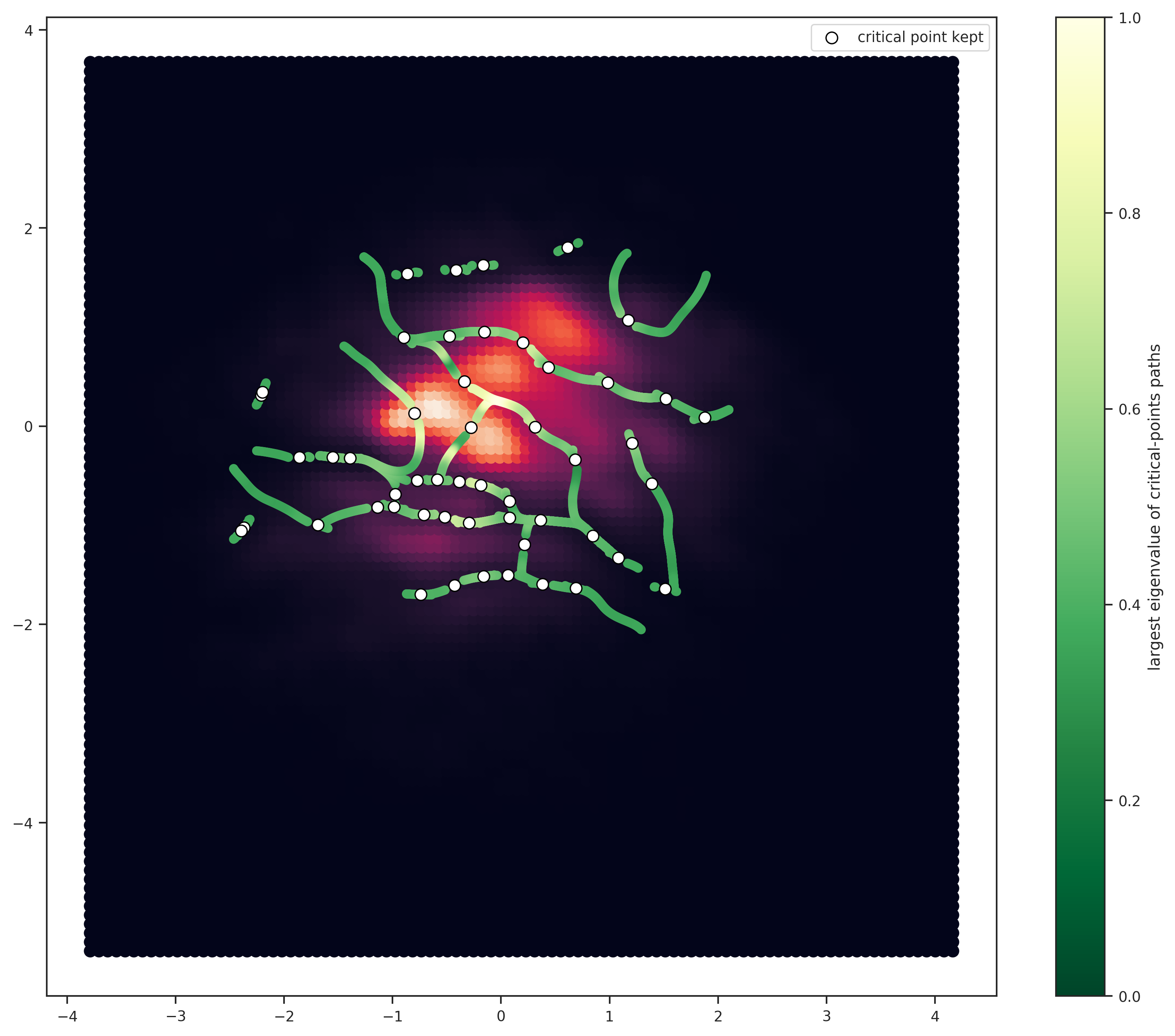
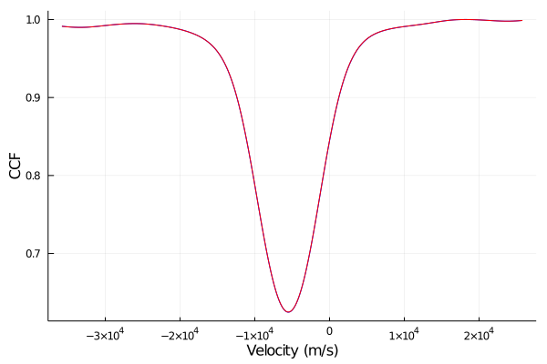
Eric showed some CCFs, CCF minus mean CCF residuals, sample covariance of CCFs, and residuals to the rank-reduced CCF covariance model, and the mean along offset diagonals of the residuals to the rank-reduced CCF covariance model, so as to give people a sense for what the data is like.

Someone (Hogg?) asked why Eric needed to compute the covariance of the CCF in the first place. Eric replied that he was trying to use the CCF for a log likelihood that was sensitive to the line-shape changes due to stellar variability.

Eric presented the above options, hoping that someone would point out some papers where scientists had thought about this more deeply and validated one or more approximations. Unfortunately, we didn’t identify any such paper. It’s unclear what subbranch of astronomy would care about computing the covariance of the CCF accurately. Maybe there’s some other field using CCFs that would care (e.g., MRIs?).
For now, it seems that the CCF covariance approximation of 5 is state-of-the-art, at least for large datasets. If Eric manages to try the bootstrap approach, he’ll report back.

References Footnotes

1. Bouchy et al. (2001)
2. Boisse et al. (2010)
3. Lafarga et al. (2020)
4. For instruments using a gas absorption cell as a wavelength calibration, the velocity measurements are typically done using something closer to a forward modeling approach; Butler et al. (1996). The advent of optical laser frequency combs (LFCs) and etalons has enabled even more precise wavelength calibration that can leave the stellar spectrum unperturbed.
5. Collier-Cameron et al. (2020)
6. Dumusque et al. 2020; actually we used 910 daily average spectra from this data set, rather than all 34,550 solar spectra. The daily averages have very high SNR, ~6,000-10,000 per CCF “pixel”.
7. Technically, one would need to do 6 dimensional integrals if one were to consider the finite extent of each detector pixel.

About the author:

Eric Ford has been joining in on the CCA’s Astro Data group meetings while on sabbatical, and is eager to learn from others at CCA applying advanced statistical or data science methodologies that may be relevant to detecting and characterizing exoplanets and exoplanet populations.

At this week’s meeting, I asked the group for some advice about coding in Julia vs. in Python. I am starting work on a project with David Spergel and Ruth Angus, simulating the exoplanet astrometry yield from the Nancy Grace Roman Space Telescope. We are going to look at synergies between Roman exoplanet astrometry and radial velocity (RV) observations from the Terra Hunting Experiment. In order to simulate the joint RV and astrometry signals, we are planning on using exoplanet or The Joker as well as some other exclusively Python packages. So, I asked for advice on whether it would still be “worth it” in terms of computational speed to write the code in Julia if the code I am writing will be primarily a wrapper for other Python packages. In addition, I was curious whether calling Python packages in Julia (using PyCall) would introduce a slowdown in the code.

Eric Ford said that there is no speed penalty in using PyCall in order to run Python packages in Julia. He also mentioned that Python actually works quite well as a scripting language, so if I will primarily be calling Python packages for the meat of the code, then it would work well to do so in Python. The conversation then turned into a deeper discussion about the possible benefits/downsides of re-implementing the existing Python packages in Julia. Dan Foreman-Mackey suggested that the codes themselves are quite replicable and it wouldn’t be too difficult to re-implement them in Julia. David Hogg brought up the benefit in writing my own code from scratch in terms of developing a deeper understanding of how the code works. He also suggested for me to “think about your goals and do what makes sense within those goals.” Megan Bedell and Adrian Price-Whelan then suggested an alternative approach could be to implement a few toy or simpler cases to get a feel for what’s going on, but ultimately using existing packages in production work. Dan Foreman-Mackey also mentioned that the Julia code wouldn’t be quicker than the existing Python packages, as these packages use C or C++ for the computationally expensive portions of the code.

The main takeaway I got from the conversation is that it would be possible to do the project in Julia, by re-writing the Python packages that I would need, but that this is only really the right approach if it is something that I am specifically interested in doing as a project in itself. Otherwise, if the primary goal is to quickly produce a functioning simulation of Roman astrometry + Terra Hunting RVs, then it is likely better to use the existing Python code bases and to write the wrapping/scripting code in Python as well.

Figure credit

At this week’s meeting I updated the group on an ongoing project examining the influence of age on the exoplanet radius gap, a relative scarcity of close-in exoplanets sized between 1.5-2 Earth radii. The feature is widely believed to be a signature of atmospheric loss, with planets below the gap having rocky compositions and planets above the gap requiring a few percent-by-mass atmospheres to explain their low bulk densities. In the atmospheric loss paradigm, some fraction of the rocky planets are the remnant cores of planets that lost the entirety of their atmospheres.

At the core of this project is the observation of a more sparsely populated radius gap at younger system ages. My question to the group was in regards to estimating the statistical significance of the feature in 1D (i.e. just the radius distribution) and 2D (i.e. the orbital period-radius plane). While the gap appears to be remarkably empty in 2D, the feature is somewhat washed out (or, less statistically significant) in 1D partially due to the fact that the precise location of the gap decreases with increasing orbital period. In the 1D case, David W. Hogg proposed that the data could be projected orthogonally to an assumed functional form of the gap. A grid search of the gap function parameters could be performed to test different projections and find the “best” or emptiest gap, which would also allow us to estimate the feature’s significance through simulations.

Christina Hedges brought up Hough transforms for the 2D case. Since there also appears to be a stellar mass dependence to the location of the radius gap (and conceivably a metallicity dependence), we would be interested in exploring the location of the gap in higher dimensions. Generalizing the Hough transform to higher dimensions was discussed, and Christina threw together a lovely notebook for the 2D case.

At this week’s meeting, I updated the group about my project with D F-M, Andy Casey (Monash University), and Tim Morton (USC- the west coast one). We are looking into how to determine how the binarity of Kepler planet hosts influence planet formation. That sounds really exciting but “determine” is doing a lot of work in that sentence. First, we have to figure out which stars are (unresolved) binaries. There are a couple of different ways in which we’ll go about doing this, but the one highlighted this week is the fruit of Andy’s work.

Alongside the astrometric and RV measurements, Gaia also lists errors associated with fits. For unresolved binaries, trying to fit the astrometric or RV curve of a single star will yield an uncharacteristically large amount of error. Through Andy’s work (which I can’t claim to understand beyond the surface level), we can turn this error into a likelihood that the star is not a single star.

Incredibly, this seems to work really well! In the color-magnitude diagram above of the KIC stars with astrometric measurements, we can pick out the stars that have a low probability of being single above the main sequence; right where we would expect binaries to be.

Interestingly, the same plot for KIC stars with RV measurements looks very different. There are a few selection effects here we’ll have to figure out: not all stars have both astrometric and RV measurements and (as pointed out by Trevor) the population of binaries detected by astrometry is different from that of RV binaries. Known spectroscopic and eclipsing binaries are picked up through RV jitter but not astrometric jitter!

Figuring out how exactly accurate this is will be key. Because neither method is batting 1.000, exactly how to quantify “I’m pretty sure this star is not a single” represents an interesting puzzle for our near-future selves.