Given the current state of the world, we have been holding the Astro Data Group meeting virtually for the past couple of months and this blog has taken a hit over that time. This week, I (Dan) have decided to try to start posting a short summary of what we talk about each week so we’ll see how long I keep it up :)!
Fran Bartolić started us off with a discussion of how he is using non-negative matrix factorization to map the time variable surface of Io using occultation light curves. In particular, he’s modeling the time variable surface as a linear combination of starry maps where the coefficients vary as a function of time. The results of this inference are prior dependent so he presented some of the prior information that he is considering: non-negativity constraints, sparsity priors, and Gaussian processes to capture smooth time variability and volcano duty cycles. There was some discussion about including spatial priors that would favor contiguous features in each map (for example, individual volcanos).
Trevor David has been investigating long run times and divergences in his PyMC3 inferences. To handle difficult posterior inferences, he has been increasing the target acceptance statistic in the tuning phase of his PyMC3 runs, but still ends up with some small percentage of diverging samples and long run times. Some of these issues can be handled by re-parameterization, but Trevor has been looking at various diagnostics to try and understand the behavior of his sampler. One such diagnostic is the comparison of the empirical marginal energy distribution and the conditional energy distribution (see figure 23 of Betancourt 2017 for an example), and Trevor finds a small skew in these distributions (with heavier tails to larger energies).
On a related topic, I presented some work I have been doing to improve the tuning performance for PyMC3 when there is a large dynamic range in posterior precision across dimensions. The idea is fairly simple—set the target acceptance statistic to something low (like 50%) at the beginning of the tuning phase and increase this target to the final value throughout tuning—but it seems to work well for at least some test cases. This is currently implemented in exoplanet, but more testing will be needed before this is ready for prime time.
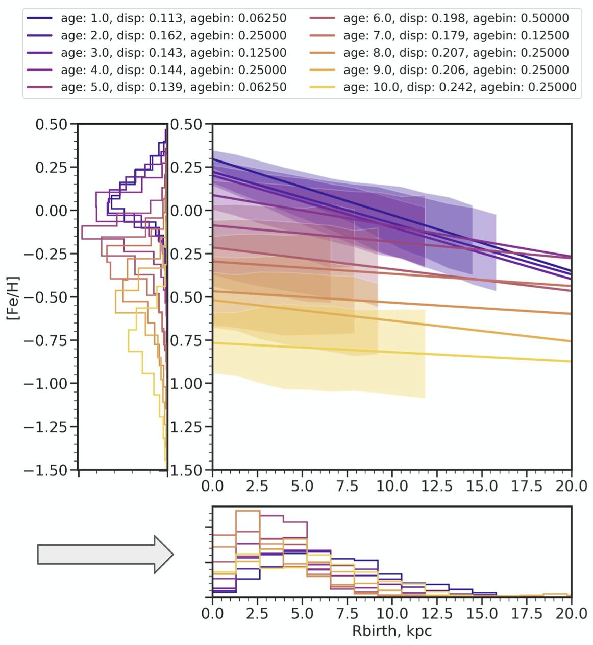
Dreia Carrillo shared the figure at the top of this post and asked for feedback about its clarity and, in particular, the binning choices made in the bottom histogram. This figure shows stellar metallicity gradients as a function of birth radius in a Milky Way-like galaxy simulation. The main panel shows how these gradients change as a function of age, but doesn’t capture underlying density of stars so she included the histograms to show this distribution, and specifically to highlight the signatures of inside-out disk formation. The group discussed options for making the birth radius histogram plot clearer. These suggestions included using a kernel density estimate instead of a histogram and using fewer, wider age bins.
To finish, Emily Cunningham led a discussion of how members of the group manage their time when working on multiple parallel projects and how to identify when we are over-committed to too many projects. The group agreed that this is something we all struggle with, especially since we are currently all working in isolation. Group members have devised some tactics for dealing with this, including setting goals on week-long time scales instead of daily or by running work by collaborators more frequently. We also discussed the fact that side projects and context switching can be useful (especially these days) to help getting ourselves out of a research rut or to identify our next projects, even if they don’t always lead to visible results.