The stellar halo of the Milky Way is full of debris streams — “stellar streams” — left over from dwarf galaxies and globular clusters that have been destroyed by our Galaxy’s gravitational field. These structures are diffuse, distant, and much lower density than foreground stars in, e.g., the Milky Way disk, which is why they don’t appear if you just plot the sky positions of all stars from a photometric survey like the SDSS or Pan-STARRS. One way to search for and enhance the significance of stellar streams is to filter photometric data using templates constructed from isochrones of stellar populations that have characteristics similar to the typical objects that we think disrupt to form the streams (typically low metallicity and old). By moving these color-magnitude filters in distance or distance modulus, we can then construct density maps of the sky positions of these filtered stars to look for linear features that persist or appear consistent between different distance slices. This has been done in the past using, e.g., the northern SDSS data, the full SDSS footprint, and Pan-STARRS.
This week, Nora Shipp (Chicago; who found most of the known streams in the southern sky) has been visiting the CCA to search for new streams, and confirm the existence of stream candidates, using data from the DESI Imaging Legacy Surveys. This survey is deeper and higher resolution than the SDSS, so we are hoping we will find some interesting new things. So far, we have produced filtered sky-maps in distance slices, and are beginning to correlate structures in our new maps with past surveys and discoveries.
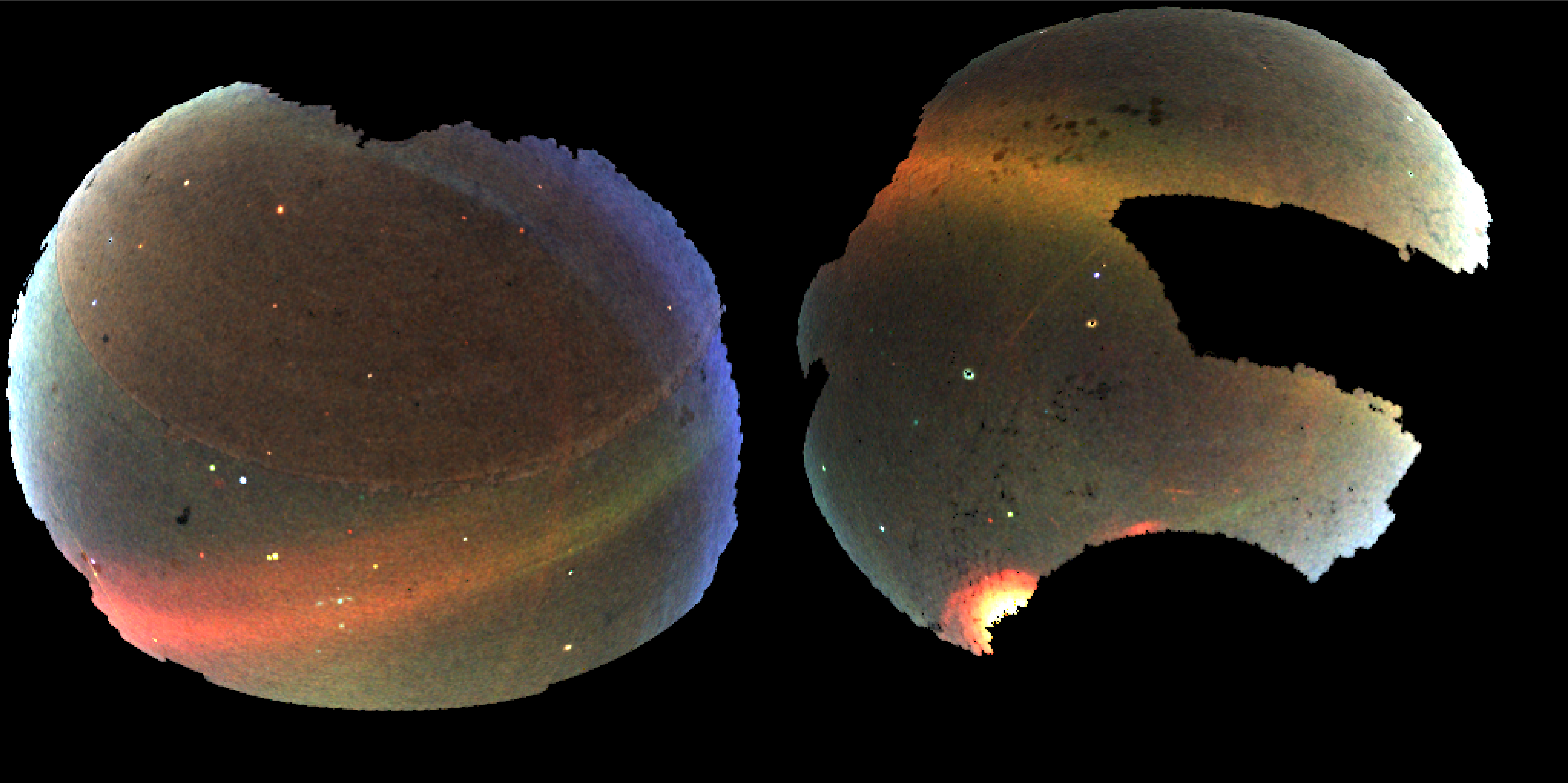
One way of visualizing the data is to produce a “field of streams” map, by assigning density in different distance slices to different color channels. In the sky map figure shown above (in equatorial coordinates), the intensity of each pixel is related to the number of stars that pass our color-magnitude filter, and the color of each pixel is an indication of the mean distance of stars in that pixel. In this case, red pixels are ~20–60 kpc from the sun, green is ~10–20 kpc, and blue is ~5–10 kpc. Already with this map, we can see many of the known prominent streams in the northern and southern hemispheres (the widest and most prominent being the Sagittarius stream). Now that we have pretty images, we have to buckle down and try to characterize individual features!